Volatility Mean Reversion: A Systematic Approach to Premium Selling

1. Executive Summary

Implied volatility exhibits a robust statistical tendency to revert to its historical mean, presenting a compelling edge for sophisticated options traders. This report details a systematic premium-selling strategy that quantifies mean reversion speed, identifies optimal entry points using Implied Volatility Rank (IVR) and Z-scores, and outlines precise trade construction, risk management, and historical validation to capitalize on this persistent market anomaly.

2. The Anomaly Explained

What is Volatility Mean Reversion?

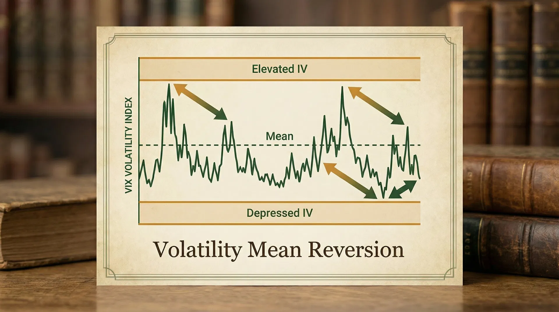
Volatility mean reversion refers to the observed phenomenon where both historical and implied volatility tend to return to their long-term average levels over time. Unlike asset prices, which can trend indefinitely, volatility is inherently bounded and cyclical. Periods of high volatility are typically followed by periods of lower volatility, and vice versa. This statistical property is a cornerstone for many options trading strategies, particularly those focused on selling premium. The underlying principle is that extreme deviations in implied volatility from its historical norm are unsustainable and will eventually correct. This differs fundamentally from price mean reversion, where an asset's price may revert to a moving average, but the underlying asset can still experience significant long-term price appreciation or depreciation. Volatility, however, is a measure of the rate of price change, and this rate tends to oscillate around a stable equilibrium [1].

Why Does it Exist?

The mean-reverting nature of volatility is driven by a confluence of market microstructure, behavioral finance, and institutional hedging activities. From a market microstructure perspective, periods of high volatility often trigger increased trading activity, leading to wider bid-ask spreads and higher option premiums. As uncertainty subsides, liquidity improves, and bid-ask spreads narrow, causing implied volatility to decline. Conversely, during periods of low volatility, complacency can set in, leading to reduced hedging demand and lower option prices. Any sudden shock can then cause a rapid spike in volatility as market participants rush to hedge or speculate, initiating the reversion cycle [2].

Behavioral finance also plays a significant role. Traders and investors often overreact to news and events, leading to exaggerated movements in implied volatility. Fear and greed can push implied volatility to extreme highs or lows, creating temporary mispricings that rational market participants eventually correct. This overreaction and subsequent correction contribute to the observed mean-reverting behavior.

Furthermore, the hedging activities of institutional players, such as market makers and portfolio managers, contribute to volatility mean reversion. Market makers, who are constantly delta-hedging their option books, tend to buy volatility when it's low and sell it when it's high to maintain a balanced risk profile. This continuous rebalancing acts as a natural dampener on extreme volatility movements. Similarly, portfolio managers often purchase portfolio insurance (e.g., put options) during periods of perceived high risk, driving up implied volatility. As market conditions stabilize, this demand wanes, allowing volatility to revert. The collective actions of these participants create a powerful force that pulls implied volatility back towards its historical average [3].

3. Identifying the Setup

Quantifying Mean Reversion Speed

Quantifying the speed at which implied volatility reverts to its mean is crucial for developing a systematic trading strategy. While there isn't a single universally accepted metric, several approaches can provide valuable insights. One common method involves analyzing the half-life of volatility, which is the time it takes for volatility to halve its deviation from its long-term mean. This can be estimated using econometric models, such as an Ornstein-Uhlenbeck process, which is often used to model mean-reverting processes. Alternatively, a simpler, empirical approach involves observing historical data to determine the average duration of volatility spikes and troughs and the subsequent return to the mean. For instance, analyzing the VIX index, it has been observed that extreme spikes tend to revert relatively quickly, often within weeks or a few months [4].

Another practical way to gauge mean reversion speed is to examine the historical behavior of IVR and IVP. By backtesting various thresholds and observing how quickly implied volatility moves from extreme levels back towards its average, traders can develop a qualitative understanding of the mean reversion speed for specific underlying assets. Faster mean reversion implies more frequent trading opportunities and potentially shorter holding periods for premium-selling strategies.

Implied Volatility Rank (IVR) and Percentile (IVP)

Implied Volatility Rank (IVR) and Implied Volatility Percentile (IVP) are indispensable tools for options traders seeking to capitalize on volatility mean reversion. Both metrics provide a contextual understanding of an asset's current implied volatility relative to its historical range over a specified period, typically the past 52 weeks.

IVR is a simple calculation that expresses the current implied volatility as a percentage of its range between the 52-week high and 52-week low. An IVR of 0% indicates that the current implied volatility is at its 52-week low, while an IVR of 100% signifies it's at its 52-week high. An IVR above 50% generally suggests that implied volatility is relatively high, making it a potentially opportune time to sell premium [5].

IVP, on the other hand, reports the percentage of days over the last 52 weeks that implied volatility traded below the current level. For example, an IVP of 90% means that implied volatility has been lower than its current level 90% of the time over the past year. This indicates that current implied volatility is in the upper 10% of its historical range, again suggesting a favorable environment for selling options [5].

Both IVR and IVP are valuable because they normalize implied volatility, allowing for comparisons across different assets and over time. A high IVR or IVP signals that options are relatively expensive, offering a higher premium for sellers, and that implied volatility is likely to revert downwards, benefiting short volatility positions.

Z-Scores for Optimal Entry Points

While IVR and IVP provide a relative measure of implied volatility, Z-scores offer a statistical measure of how far the current implied volatility deviates from its historical mean in terms of standard deviations. This provides a more precise quantification of the extremity of the current implied volatility. The formula for a Z-score is:

Z = (Current IV - Mean IV) / Standard Deviation of IV

Where: * Current IV is the current implied volatility. * Mean IV is the historical average implied volatility over a defined period (e.g., 1 year). * Standard Deviation of IV is the historical standard deviation of implied volatility over the same period.

A high positive Z-score (e.g., +1.5 or +2.0) indicates that the current implied volatility is significantly above its historical average, suggesting that options are overpriced and ripe for premium selling. Conversely, a low negative Z-score would indicate undervalued options. Using Z-scores helps traders identify statistically significant deviations, reducing subjective judgment and providing a data-driven trigger for trade entry [6].

Specific Quantitative Criteria

For a systematic premium-selling strategy based on volatility mean reversion, precise quantitative criteria are essential for identifying high-probability setups. These criteria typically include:

• Implied Volatility Rank (IVR) / Percentile (IVP): A minimum IVR or IVP threshold, often above 50% or 70%, indicates that implied volatility is elevated and likely to revert downwards. Higher thresholds generally imply greater premium and a stronger mean reversion edge.
• Z-Score of Implied Volatility: A positive Z-score, typically above +1.0 or +1.5, confirms that the current implied volatility is statistically significantly above its historical mean, reinforcing the mean reversion signal.
• Days to Expiration (DTE) Window: Options with shorter DTE (e.g., 30-60 days) tend to exhibit faster time decay (theta), which benefits premium sellers. However, very short-dated options (e.g., < 21 DTE) can be more susceptible to gamma risk. An optimal window often falls between 30 and 75 DTE.
• Delta Ranges for Short Options: For selling strategies like iron condors, selecting short strikes with a delta between 10 and 30 (absolute value) provides a balance between collecting sufficient premium and maintaining a high probability of out-of-the-money expiration. This corresponds to a higher probability of profit, typically above 70%.
• Underlying Asset Liquidity: The underlying stock or ETF must have sufficient liquidity in its options market to ensure efficient entry and exit without significant slippage. High average daily volume and tight bid-ask spreads are critical.
• Market Conditions: While volatility mean reversion is a robust anomaly, it performs best in range-bound or moderately trending markets. Avoid initiating large premium-selling positions during periods of extreme market uncertainty or strong directional trends, as these can lead to sustained high volatility or rapid price movements that overwhelm the mean reversion effect.

4. Trade Construction

For a systematic premium-selling strategy, the Iron Condor is a highly favored options structure due to its defined risk and ability to profit from both decreasing volatility and time decay. An Iron Condor involves selling an out-of-the-money (OTM) call spread and an OTM put spread on the same underlying asset and expiration date. The goal is for the underlying price to remain between the short strikes at expiration.

Iron Condor Example

Consider a hypothetical scenario for Ticker: SPY (S&P 500 ETF) with the following market conditions:

• Current SPY Price: $500
• Implied Volatility Rank (IVR): 80% (indicating high IV)
• Implied Volatility Z-Score: +1.8 (indicating statistically high IV)
• Days to Expiration (DTE): 45 days

Trade Structure: Sell 45-Day SPY Iron Condor

• Sell Put Spread:
  • Sell 1 SPY 480 Put (Delta -0.20)
  • Buy 1 SPY 475 Put (Delta -0.15)
  • Credit Received for Put Spread: $1.20
• Sell Call Spread:
  • Sell 1 SPY 520 Call (Delta +0.20)
  • Buy 1 SPY 525 Call (Delta +0.15)
  • Credit Received for Call Spread: $1.10

Total Credit Received (Premium): $1.20 + $1.10 = $2.30 (or $230 per contract)

Maximum Potential Loss: The width of the spread minus the credit received. In this case, the width of each spread is $5.00 ($480-$475 or $525-$520). So, Max Loss = $5.00 - $2.30 = $2.70 (or $270 per contract).

Breakeven Points at Expiration: * Lower Breakeven: Short Put Strike - Total Credit = $480 - $2.30 = $477.70 * Upper Breakeven: Short Call Strike + Total Credit = $520 + $2.30 = $522.30

Probability of Profit (POP): This can be estimated using the deltas of the short options. With short deltas around 0.20, the approximate POP for each side is 80%. For the entire iron condor, the POP is typically higher than a single short option, often in the range of 65-75%, depending on the spread width and credit received. For this example, let's assume a POP of 70%.

5. Entry/Exit Rules

Precise entry and exit rules are paramount for systematically exploiting volatility mean reversion and managing risk effectively.

Entry Rules

1. IVR/IVP Threshold: Enter a premium-selling trade (e.g., Iron Condor) only when the underlying asset's Implied Volatility Rank (IVR) is above 70% or Implied Volatility Percentile (IVP) is above 80%. This ensures that implied volatility is significantly elevated, offering attractive premium.
2. IV Z-Score Confirmation: Confirm the high IV environment with an Implied Volatility Z-score greater than +1.5. This provides statistical validation that current IV is an outlier and likely to revert.
3. Days to Expiration (DTE): Select an expiration cycle with 30 to 75 Days to Expiration. This window balances sufficient time decay with manageable gamma risk.
4. Delta Selection: For Iron Condors, sell the out-of-the-money (OTM) options with absolute deltas between 0.15 and 0.25. This targets a high probability of profit (typically 75-85% for each spread leg) while collecting reasonable premium.
5. Liquidity Check: Ensure the underlying asset and its options have ample liquidity (tight bid-ask spreads, high open interest) to facilitate efficient order execution.

Profit Taking

• Target 50% of Max Profit: Systematically close the entire Iron Condor position when 50% of the maximum potential profit (i.e., 50% of the credit received) has been realized. This rule captures profits efficiently and reduces exposure to adverse movements as expiration approaches. For our example, this would be closing the trade when the position value drops by $1.15 ($2.30 * 0.50).

Stop Loss

• 1x Max Loss: Close the entire Iron Condor position if the unrealized loss reaches 1x the maximum potential loss. This is a critical risk management rule to prevent catastrophic losses. For our example, this would be closing the trade if the loss reaches $2.70 ($270 per contract). Alternatively, a stop loss at 2x the credit received can also be used (e.g., $4.60 in our example), but this exposes the trade to a larger potential loss.

Rolling Strategies

Rolling an Iron Condor involves closing the existing position and opening a new one, typically further out in time and/or at different strike prices. This is done to manage challenged positions or extend profitable ones.

1. Roll Down/Up the Unchallenged Side: If one side of the Iron Condor (e.g., the put spread) is being challenged by the underlying price moving towards it, consider rolling the unchallenged side (the call spread) closer to the current price to collect additional credit and widen the breakeven points. This should only be done if the overall IVR/IVP remains high.
2. Roll Out in Time: If the underlying price is threatening a short strike, roll the entire Iron Condor position to a later expiration cycle (e.g., 30-45 days further out) to collect additional credit and give the underlying more time to revert. This often involves rolling to the same strike prices or slightly wider ones to maintain a similar risk profile.
3. Avoid Rolling for a Debit: Generally, avoid rolling a challenged position for a debit, as this increases the maximum potential loss and reduces the probability of profit. Rolls should ideally generate additional credit.

6. Risk Management

Effective risk management is paramount for the long-term success of any systematic premium-selling strategy, especially one based on volatility mean reversion. While the anomaly provides an edge, adverse market movements can still lead to significant losses if not properly managed.

Position Sizing

Position sizing is the most critical aspect of risk management. A common approach is to allocate a small percentage of total portfolio capital to each trade, typically 1-2% of capital at risk per trade. For an Iron Condor, the capital at risk is the maximum potential loss. For example, if a portfolio has $100,000 and the max loss per Iron Condor is $270, a 1% allocation would mean trading approximately 3-4 contracts ($1000 / $270 ≈ 3.7 contracts). This ensures that no single trade can severely impair the portfolio, even in the event of a maximum loss.

Correlation Risk

Trading multiple premium-selling positions across different underlying assets introduces correlation risk. If all positions are highly correlated, a broad market move can simultaneously challenge many trades, leading to larger-than-expected losses. To mitigate this:

• Diversify Across Sectors: Trade underlying assets from different economic sectors to reduce sector-specific risk.
• Diversify Across Asset Classes: Consider trading volatility products on different asset classes (e.g., equities, commodities, currencies) if available and liquid.
• Monitor Portfolio Beta: Keep track of the overall portfolio beta to the broader market. A high beta portfolio will be more susceptible to market-wide volatility spikes.

Tail Risk Scenarios

Tail risk refers to the possibility of extreme, low-probability events that can have a severe impact on a portfolio. For premium sellers, a sudden, sharp, and sustained move in the underlying asset (often accompanied by a rapid increase in implied volatility) is the primary tail risk. Strategies to manage tail risk include:

• Defined Risk Spreads: Always trade defined-risk strategies like Iron Condors, which have a capped maximum loss. Avoid naked options selling unless explicitly part of a highly sophisticated and well-capitalized strategy.
• Portfolio Hedging: Consider holding a small percentage of portfolio capital in long volatility instruments (e.g., VIX calls, long VXX) as a hedge against extreme market downturns and volatility spikes. This can offset some losses from short volatility positions during black swan events.
• Cash Allocation: Maintain a significant cash allocation in the portfolio to absorb potential losses and provide flexibility to capitalize on new opportunities after a market dislocation.

What Can Go Wrong?

Despite the statistical edge of volatility mean reversion, several factors can lead to underperformance or losses:

• Sustained Volatility Expansion: Implied volatility can remain elevated for extended periods, especially during prolonged market crises or economic uncertainty, preventing mean reversion and causing short volatility positions to suffer from negative gamma and delta exposure.
• Rapid Directional Moves: A swift and significant move in the underlying asset, even if implied volatility is high, can quickly push an Iron Condor past its breakeven points, leading to maximum loss. This is particularly true for earnings announcements or unexpected news events.
• Liquidity Drying Up: During extreme market stress, liquidity in options markets can evaporate, making it difficult to exit challenged positions at reasonable prices.
• Over-Leverage: Excessive position sizing or using too much leverage can amplify losses and lead to margin calls, even with a statistically sound strategy.
• Model Risk: Relying solely on quantitative models without understanding their limitations or adapting to changing market regimes can lead to unexpected drawdowns.

7. Historical Context / Backtesting Evidence

Extensive academic research and empirical studies consistently demonstrate the existence and profitability of the volatility risk premium, which is the core anomaly exploited by premium-selling strategies. Historically, implied volatility has tended to be higher than realized volatility, meaning options prices generally overestimate future price movements. This persistent overestimation creates a statistical edge for options sellers [7].

Backtesting evidence for systematic premium-selling strategies, particularly those employing Iron Condors in high IV environments, often reveals attractive risk-adjusted returns. Studies by firms like tastytrade (formerly tastyworks) and various independent researchers have shown:

• Win Rates: High win rates, often in the range of 60-75%, for strategies that sell options with high IVR/IVP and manage positions actively.
• Average Returns: Consistent positive average returns over long periods, outperforming buy-and-hold equity strategies on a risk-adjusted basis.
• Sharpe Ratios: Favorable Sharpe ratios, indicating superior returns per unit of risk, especially when compared to traditional asset classes. This is often attributed to the non-correlated nature of volatility-selling profits to equity market returns.

It is crucial to note that backtesting results are hypothetical and do not guarantee future performance. However, the robustness of the volatility risk premium across different market cycles and asset classes provides a strong theoretical and empirical foundation for these strategies. Traders should conduct their own backtesting and due diligence, considering factors like transaction costs, slippage, and capital efficiency.

8. ASCII/Text Diagram

Diagram 1: Iron Condor Payoff Diagram

          Profit
            ^
            |
            |
            |       /\ 
            |      /  \ 
            |     /    \ 
            |    /      \ 
            |   /        \ 
            |  /          \ 
            | /            \ 
------------+---------------------> Price at Expiration
            | \            / 
            |  \          / 
            |   \        / 
            |    \      / 
            |     \    / 
            |      \  / 
            |       \/ 
            |
            v
          Loss

Short Put  Long Put    Short Call  Long Call
Strike     Strike      Strike      Strike

Description: This diagram illustrates the typical payoff profile of an Iron Condor at expiration. The strategy profits when the underlying asset's price remains between the two short strike prices, with maximum profit achieved when the price is between the long strikes. Losses are capped beyond the long strikes.

Diagram 2: Implied Volatility Z-Score Distribution

          Frequency
              ^
              |
              |
              |       /\ 
              |      /  \ 
              |     /    \ 
              |    /      \ 
              |   /        \ 
              |  /          \ 
--------------+---------------------> Z-Score of Implied Volatility
            -2.0 -1.0  0  +1.0 +2.0

*Normal Distribution Curve*

Description: This diagram represents a normal distribution of implied volatility Z-scores. A Z-score of 0 indicates IV is at its historical mean. Positive Z-scores (e.g., +1.0, +2.0) indicate IV is above its mean, suggesting opportunities for premium selling. Negative Z-scores indicate IV is below its mean.

9. Real Trade Example

Let's walk through a real-world (hypothetical) trade example for SPY to illustrate the systematic approach.

Date: January 15, 2026

Market Conditions: * SPY Price: $485.00 * IVR: 85% (High) * IV Z-Score: +2.1 (Statistically very high) * Market Sentiment: Elevated uncertainty due to upcoming economic data.

Trade Entry (January 15, 2026):

Based on the high IVR and Z-score, we decide to sell an Iron Condor with 40 DTE (February 24, 2026 expiration).

• Sell Put Spread:
  • Sell 1 SPY Feb 24, 2026 460 Put (Delta -0.18)
  • Buy 1 SPY Feb 24, 2026 455 Put (Delta -0.13)
  • Credit Received for Put Spread: $1.10
• Sell Call Spread:
  • Sell 1 SPY Feb 24, 2026 510 Call (Delta +0.17)
  • Buy 1 SPY Feb 24, 2026 515 Call (Delta +0.12)
  • Credit Received for Call Spread: $1.05

Total Credit Received: $1.10 + $1.05 = $2.15 ($215 per contract)
Max Loss: $5.00 (spread width) - $2.15 = $2.85 ($285 per contract)
Breakeven Points: Lower: $460 - $2.15 = $457.85; Upper: $510 + $2.15 = $512.15
Initial POP: Approximately 72%

Trade Progression:

• January 29, 2026 (14 days later, 26 DTE remaining):
  • SPY Price: $490.00 (moved slightly up, but within the body of the condor)
  • Implied Volatility: Has decreased significantly, and the IVR is now 40% (mean-reverted).
  • Position Value: The Iron Condor is now trading at a debit of $1.05. This means the unrealized profit is $2.15 (initial credit) - $1.05 (current debit) = $1.10.
  • Profit Target Met: $1.10 profit represents approximately 51% of the maximum potential profit ($1.10 / $2.15 = 0.51). According to our profit-taking rule, we close the trade.

Trade Exit (January 29, 2026):

• Buy to Close Iron Condor for $1.05 debit.
• Net Profit: $2.15 (credit received) - $1.05 (debit paid) = $1.10 ($110 per contract).

This example demonstrates how the strategy profits from the mean reversion of implied volatility and time decay, allowing for a quick and efficient profit capture when the profit target is met.

10. Key Takeaways

• Volatility is Mean-Reverting: Implied volatility consistently reverts to its historical average, creating a persistent edge for options sellers.
• IVR and Z-Scores are Key: Utilize Implied Volatility Rank (IVR) and Implied Volatility Z-scores to objectively identify statistically high implied volatility environments for optimal entry.
• Systematic Entry/Exit Rules: Adhere to predefined quantitative criteria for trade entry (IVR, Z-score, DTE, Delta) and strict profit-taking (50% of max profit) and stop-loss (1x max loss) rules.
• Iron Condors for Defined Risk: Employ defined-risk strategies like Iron Condors to capitalize on volatility mean reversion while capping potential losses.
• Robust Risk Management: Implement rigorous position sizing, diversify across uncorrelated assets, and consider tail risk hedges to protect capital and ensure long-term strategy viability.

References

[1] Mean Reversion Strategies: Introduction, Trading, Strategies and More – Part I. Interactive Brokers. https://www.interactivebrokers.com/campus/ibkr-quant-news/mean-reversion-strategies-introduction-trading-strategies-and-more-part-i/
[2] Timing Mean Reversion Using Implied Volatility. CrackingMarkets. https://www.crackingmarkets.com/iv-mean-reversion/
[3] Implied Volatility (IV) Rank & Percentile Explained. tastytrade. https://www.tastylive.com/concepts-strategies/implied-volatility-rank-percentile
[4] How to approximate the time to mean reversion for implied volatility. Quant StackExchange. https://quant.stackexchange.com/questions/16738/how-to-approximate-the-time-to-mean-reversion-for-implied-volatility
[5] Implied Volatility (IV) Rank & Percentile Explained. tastytrade. https://www.tastylive.com/concepts-strategies/implied-volatility-rank-percentile
[6] Scoring Implied Volatility. Red Pill Quants. https://redpillquants.com/scoring-implied-volatility/
[7] The Benefits of Systematically Selling Volatility. RiverPark Funds. https://www.riverparkfunds.com/assets/pdfs/news/Structural_Alpha_White_Paper_Final.pdf