Skew/Smile Distortions: Trading Put Skew and Volatility Smile Anomalies

Executive Summary

The options market consistently overprices downside protection, creating a persistent anomaly known as put skew. This report delves into the mechanics of volatility skew and smile, demonstrating how sophisticated options traders can identify extreme skew conditions using 25-delta risk reversals. We will outline actionable strategies to construct trades that capitalize on the inevitable normalization of this skew, offering a systematic approach to generating consistent returns while managing inherent risks.

The Anomaly Explained

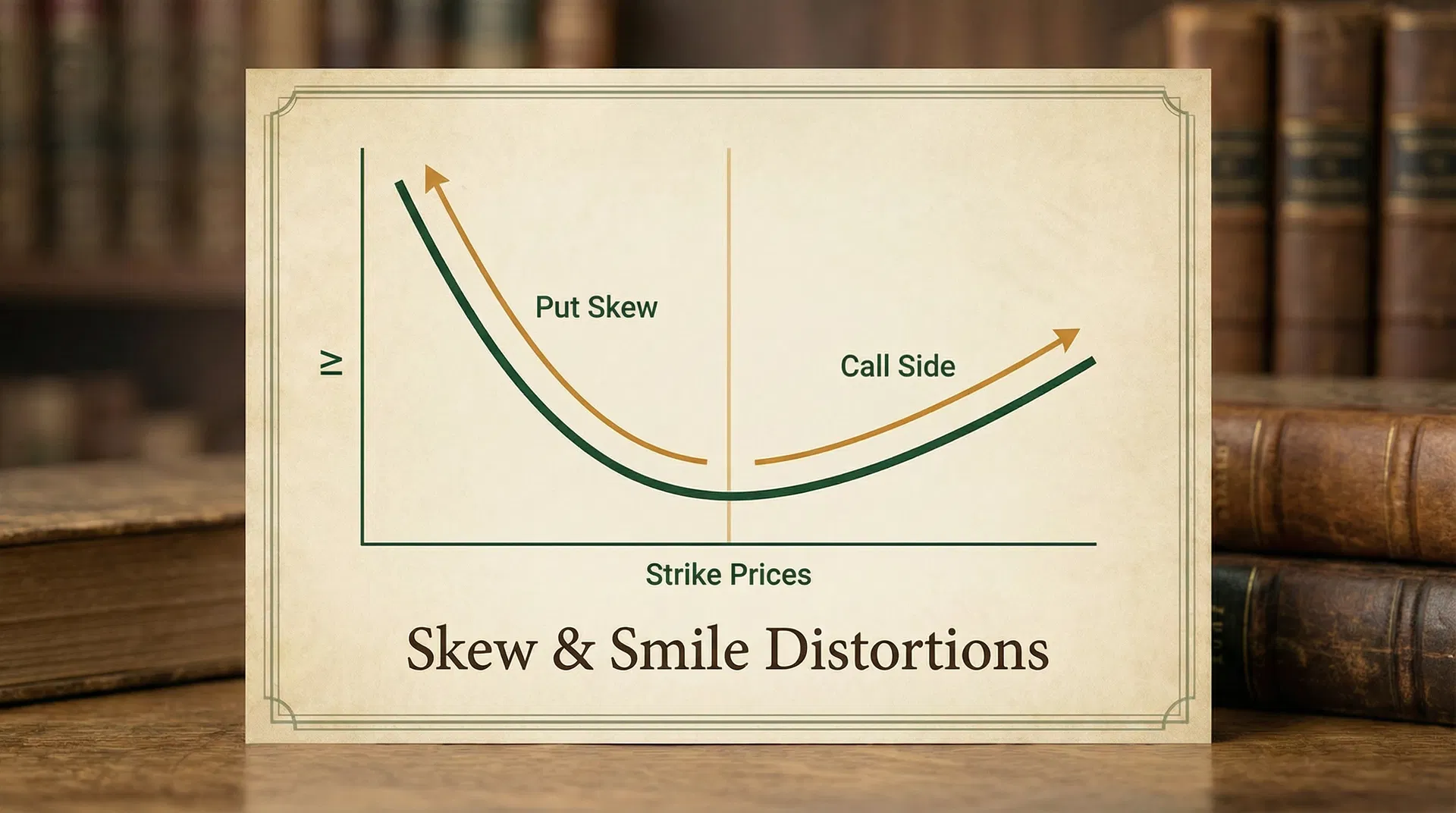
Volatility skew, often visualized as a 'smile' or 'smirk' on a graph of implied volatility (IV) against strike prices, is a fundamental characteristic of options markets. For equity indices and most individual stocks, this typically manifests as negative skew, where out-of-the-money (OTM) put options have higher implied volatilities than at-the-money (ATM) options, and OTM call options have lower implied volatilities [1]. This phenomenon is not random; it is a direct consequence of market participants' collective behavior and structural biases.

The primary driver of negative skew is the persistent demand for downside protection. Institutional investors, portfolio managers, and even retail traders frequently purchase OTM put options to hedge against potential market downturns or significant price drops in their holdings. This constant buying pressure inflates the implied volatility of OTM puts, making them relatively more expensive than their OTM call counterparts. Conversely, there is generally less demand for OTM calls, as investors are often content to let their long equity positions appreciate without additional leverage, or they might sell covered calls, which adds supply to the OTM call market, further depressing their IVs [2].

Another contributing factor is the leverage inherent in equity markets. A sharp decline in stock prices can trigger margin calls, forced selling, and a general deleveraging cascade, exacerbating market falls. Options traders price this tail risk into OTM puts, demanding a higher premium for bearing the risk of extreme downside moves. This asymmetric perception of risk—where large downside moves are considered more probable and impactful than equally large upside moves—is deeply embedded in the options pricing structure.

The market microstructure also plays a role. Market makers, who facilitate options trading, must manage their own risk exposures. When there is a consistent bid for OTM puts, market makers become structurally short volatility on the downside. To hedge this exposure, they may sell OTM calls or buy underlying stock, but often they simply widen spreads or increase the implied volatility of the puts they are selling to compensate for the increased risk [3]. This dynamic further entrenches the negative skew.

Identifying the Setup

Identifying extreme skew conditions is crucial for profitably trading this anomaly. One of the most effective tools for this is the 25-delta risk reversal. The 25-delta risk reversal (25d RR) is calculated as the implied volatility of the 25-delta call option minus the implied volatility of the 25-delta put option for a given expiration. A negative 25d RR indicates that 25-delta puts are more expensive than 25-delta calls, which is typical for equity markets. The magnitude of this negative value signifies the degree of put skew [4].

For instance, if the 25-delta call has an IV of 20% and the 25-delta put has an IV of 25%, the 25d RR is 20% - 25% = -5%. A more negative value, such as -8% or -10%, suggests a more pronounced put skew, indicating that downside protection is unusually expensive. Traders look for instances where the 25d RR reaches historical extremes, suggesting an overextension of the market's fear premium.

Specific quantitative criteria for identifying a trade setup include:

• IVR Levels: Look for underlying assets with Implied Volatility Rank (IVR) above 50%, ideally above 70%. High IVR suggests that current implied volatility is elevated relative to its historical range, making premium selling strategies more attractive.
• Delta Ranges: Focus on options with deltas around 25 for the OTM puts and calls, as this is the standard for calculating risk reversals and represents a sweet spot for capturing skew premium without excessive directional exposure.
• DTE Windows: Target options with 30 to 60 Days to Expiration (DTE). This window provides sufficient time for theta decay to work in your favor while avoiding the extreme volatility and gamma risk associated with very short-dated options, and the slower decay of longer-dated options.
• Skew Extremes: Identify situations where the 25d RR is at or near its historical minimum (most negative) for the chosen DTE. This can be assessed by comparing the current 25d RR to its 52-week or 1-year range. A 25d RR in the bottom 10-20% of its historical range would signal an extreme skew condition.
• Underlying Asset Characteristics: Prioritize highly liquid underlying assets, such as major equity indices (e.g., SPY, QQQ) or large-cap stocks with deep options markets. This ensures efficient execution and tighter spreads. Avoid illiquid options where bid-ask spreads can erode potential profits.

Trade Construction

A common strategy to profit from skew normalization is a risk reversal spread, often structured as selling an OTM put and buying an OTM call. When the market overprices downside protection (high put skew), selling the expensive OTM put and simultaneously buying a relatively cheaper OTM call can create a positively skewed payoff profile that benefits from the normalization of implied volatilities.

Let's consider a hypothetical example:

Example: Trading Skew Normalization in SPY

Assume SPY is trading at $450. The 25-delta risk reversal for the 45 DTE options is at an extreme low of -8%, indicating significant put skew. IVR for SPY is 75%.

Trade Structure: Sell 1 SPY 45 DTE 430 Put (approx. 25 delta) and Buy 1 SPY 45 DTE 470 Call (approx. 25 delta).

Option Leg	Strike	Delta (approx.)	Premium
Sell Put	$430	-0.25	$3.50 (credit)
Buy Call	$470	0.25	$1.50 (debit)

Net Credit Received: $3.50 - $1.50 = $2.00 per share, or $200 per contract.

Max Loss: The maximum loss on this trade is theoretically unlimited on the upside if SPY rallies significantly beyond the call strike, and substantial on the downside if SPY falls below the put strike. However, this strategy is typically managed dynamically, and the net credit received provides some buffer. The primary goal is to profit from IV normalization, not directional movement. For a pure risk reversal, the max loss on the downside is the put strike minus the credit received, and on the upside, it's theoretically unlimited beyond the call strike. However, for this specific skew normalization trade, the intention is to close the position as skew normalizes, not to hold to expiration for extreme moves.

Breakevens:

• Downside Breakeven: Put Strike - Net Credit = $430 - $2.00 = $428.00
• Upside Breakeven: Call Strike + Net Credit = $470 + $2.00 = $472.00

Probability of Profit: This depends on the implied volatility distribution. Given the extreme put skew, the probability of the underlying staying above the put strike is higher than implied by a normal distribution. The probability of profit for this specific setup would be estimated based on the distance of the breakevens from the current price, adjusted for the skew. If the underlying stays between $428 and $472, the trade is profitable. The expectation is that as skew normalizes, the implied volatility of the put will decrease, and the implied volatility of the call will increase, allowing for profitable exit before expiration.

Entry/Exit Rules

Precise entry and exit rules are paramount for consistently profiting from skew normalization strategies.

• Entry: Initiate the trade when the 25-delta risk reversal reaches an extreme negative level (e.g., in the bottom 10-20% of its 1-year range) for the chosen DTE, and the underlying asset has an IVR above 50%. Confirm that the underlying is not in an immediate, strong directional trend that could overwhelm the skew normalization effect.
• Take Profit: Aim to take profit at 50% of the maximum potential credit received. For the SPY example, this would be $1.00 per share ($100 per contract). This partial profit-taking allows for consistent wins and reduces exposure to adverse movements as expiration approaches. Alternatively, exit when the 25-delta risk reversal normalizes significantly (e.g., moves back towards its historical average).
• Stop Out: Implement a strict stop-loss. A common approach is to exit the entire position if the loss reaches 1x or 1.5x the initial credit received. For the SPY example, if the loss reaches $2.00 to $3.00 per share ($200-$300 per contract), close the trade. This prevents small losses from escalating into catastrophic ones.
• Rolling: If the trade moves against you but has not hit the stop-loss, consider rolling the position. This typically involves rolling the entire risk reversal spread to a later expiration month, potentially adjusting strikes to collect additional credit or reduce risk. Rolling should be done strategically, for instance, if the underlying has moved slightly against the position but the skew remains extreme, offering another opportunity for normalization. Avoid rolling losing positions indefinitely.

Risk Management

While skew normalization strategies offer attractive opportunities, robust risk management is essential to mitigate potential losses.

• Position Sizing: Never allocate more than 1-2% of your total trading capital to a single trade. This ensures that even if a trade goes significantly wrong, it does not materially impair your overall portfolio. Consider the capital at risk, not just the premium received.
• Correlation Risk: Be mindful of correlated assets. If you have multiple skew normalization trades on highly correlated assets (e.g., SPY and QQQ), a broad market move can impact all positions simultaneously. Diversify across uncorrelated assets or sectors where possible.
• Tail Risk Scenarios: While the strategy aims to profit from the overpricing of tail risk, extreme, unforeseen market events (e.g., a black swan event) can still lead to significant losses. Understand that selling options, even in a spread, involves inherent tail risk. Consider using defined-risk strategies or allocating a small portion of capital to long-volatility hedges if tail risk is a major concern.
• What Can Go Wrong: The primary risks include a sustained, rapid directional move against the position (either sharply up or sharply down), or the skew failing to normalize and instead becoming even more extreme. A sudden increase in overall market volatility (e.g., VIX spike) can also negatively impact the short put leg more than the long call leg, even if the relative skew remains unchanged.

Historical Context / Backtesting Evidence

The phenomenon of volatility skew, particularly the overpricing of downside protection, is well-documented and has persisted across various market cycles and asset classes. Academic research and quantitative studies consistently demonstrate that selling OTM puts, or strategies that exploit negative skew, have historically generated positive risk-adjusted returns [5]. This is often attributed to the behavioral biases of market participants (fear of crashes) and the structural demand for hedging.

While specific backtesting results for 25-delta risk reversal normalization strategies are less publicly available due to their proprietary nature, the underlying principle—that extreme deviations from historical averages tend to revert—is a cornerstone of quantitative finance. Studies on options selling strategies, particularly those focused on high IV environments, often show:

• Win Rates: Typically range from 60% to 80% for premium selling strategies, depending on the specific entry/exit criteria and risk management rules. Strategies that specifically target extreme skew conditions may exhibit higher win rates due to the statistical edge.
• Average Returns: Can vary significantly but often outperform buy-and-hold strategies on a risk-adjusted basis. The key is consistent, small gains from premium collection, punctuated by occasional losses that must be managed effectively.
• Sharpe Ratios: Strategies that effectively manage risk and capture volatility premium often exhibit favorable Sharpe ratios, indicating superior returns per unit of risk taken.

It is crucial for traders to conduct their own backtesting and forward testing on specific assets and timeframes to validate the efficacy of these strategies. Factors such as transaction costs, slippage, and liquidity can significantly impact real-world performance.

ASCII/Text Diagram

Diagram 1: Volatility Skew Profile

Implied Volatility
      ^
      |
      |      /\   (OTM Calls)
      |     /  \ 
      |    /    \ 
      |   /      \ 
      |  /        \ 
      | /          \ 
      |/____________\_________
      -------------------------> Strike Price
      OTM Puts   ATM   OTM Calls

      (Higher IV for OTM Puts, Lower IV for OTM Calls)
    

Diagram 2: Risk Reversal Payoff (Simplified)

P&L
  ^
  |
  |      /\   (Profit from Call)
  |     /  \ 
  |    /    \ 
  |   /      \ 
  |  /        \ 
  | /          \ 
  |/____________\_________
  -------------------------> Underlying Price
  (Loss from Put) (Profit from Skew Normalization) (Loss from Call)

  (Selling OTM Put, Buying OTM Call - Benefits from price moving up or skew normalizing)
    

Real Trade Example

Let's walk through a complete hypothetical trade on AAPL from entry to exit, demonstrating the application of the principles discussed.

Date: January 15, 2025

Underlying: AAPL trading at $180.00

Market Conditions:

• AAPL IVR: 80% (high)
• 45 DTE 25-delta Risk Reversal: -7.5% (historically extreme negative)

Trade Entry (January 15, 2025, 45 DTE):

Based on the extreme negative 25d RR and high IVR, a skew normalization trade is initiated.

• Sell 1 AAPL Feb 2025 170 Put (approx. 25 delta) @ $2.50 (credit)
• Buy 1 AAPL Feb 2025 190 Call (approx. 25 delta) @ $1.00 (debit)

Net Credit Received: $2.50 - $1.00 = $1.50 per share, or $150 per contract.

Max Profit Target: 50% of net credit = $0.75 per share, or $75 per contract.

Stop Loss: 1.5x net credit = $2.25 per share, or $225 per contract loss from entry.

Scenario 1: Skew Normalizes (Successful Trade)

Date: February 5, 2025 (25 DTE remaining)

Underlying: AAPL trading at $182.00

Market Conditions:

• AAPL IVR: 60% (decreased)
• 25-delta Risk Reversal: -4.0% (normalized significantly)

The implied volatility of the OTM put has decreased more than the OTM call, and the overall skew has normalized. The position is showing a profit.

• Buy 1 AAPL Feb 2025 170 Put @ $1.50 (debit)
• Sell 1 AAPL Feb 2025 190 Call @ $0.75 (credit)

Net Debit to Close: $1.50 - $0.75 = $0.75 per share.

P&L: Initial Credit ($1.50) - Debit to Close ($0.75) = $0.75 per share profit, or $75 per contract.

This meets the 50% profit target, and the trade is closed successfully.

Scenario 2: Skew Worsens / Price Moves Against (Stop Out)

Date: January 25, 2025 (35 DTE remaining)

Underlying: AAPL trading at $175.00

Market Conditions:

• AAPL IVR: 90% (increased)
• 25-delta Risk Reversal: -9.0% (skew has become even more extreme)

The market has moved against the position, and the skew has become more pronounced. The position is showing a loss exceeding the stop-loss threshold.

• Buy 1 AAPL Feb 2025 170 Put @ $4.00 (debit)
• Sell 1 AAPL Feb 2025 190 Call @ $0.50 (credit)

Net Debit to Close: $4.00 - $0.50 = $3.50 per share.

P&L: Initial Credit ($1.50) - Debit to Close ($3.50) = -$2.00 per share loss, or -$200 per contract.

This loss is within the acceptable stop-loss range of $2.25, and the trade is closed to prevent further losses.

Key Takeaways

• The options market consistently overprices downside protection, creating a persistent negative skew.
• 25-delta risk reversals are a powerful tool to identify extreme skew conditions.
• Target high IVR environments (above 50%) and 30-60 DTE for optimal trade setups.
• Construct trades by selling expensive OTM puts and buying relatively cheaper OTM calls to profit from skew normalization.
• Implement strict entry, exit, and risk management rules, including a 50% profit target and a defined stop-loss.